
Pneumonia Chest X-Ray Classification
Published:
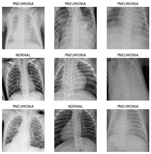
The dataset used for this task if from a Kaggle dataset by Paul Mooney. It consists of two kinds of chest x-rays, those infected by pneumonia, and the other being normal. Our main goal is to distinguish which chest corresponds to pneumonia-infected ones and which aren’t. Note that the dataset is highly imbalanced, like many medical image dataset are.
Fast.ai2 Library
Fast.ai has just released its version 2 framework. It is bundled with tons of old plus new shiny features which weren’t available previously such as its brand new medical applications. Although this task isn’t related to actually using the medical applications, it serves as a stepping-stone.
Fastbook
Aside from releasing its version 2 framework, fast.ai also released a companion-book dubbed fastbook. The book is available for free in the form of Jupyter notebooks, but one can also purchase a print version on Amazon. More importantly, this task is applying what I’ve learned from the 7th Chapter of the book called Training a State-of-the-Art Model.
Transfer Learning
Lastly, I’ve also applied Transfer Learning in this task, since I’ve seen it to perform better with it after a couple of runs. The particular model I’ll be using is EfficientNetB3A, with weights from Ross Wightman’s timm library.
Code
import torch
import fastai
from fastai.vision.all import *
from fastai.vision.core import *
from fastai.callback import *
from fastai.metrics import *
import numpy as np
from sklearn.metrics import precision_score, recall_score, confusion_matrix
import matplotlib.pyplot as plt
from timm import create_model
Load Data
The dataset is very imbalanced. Firstly, it has more pneumonia-infected chest x-rays compared to normal ones. Regardless, I’ve tried to oversample using PyTorch’s WeightedRandomSampler as it didn’t show much of an improvement. Secondly, it has a very small validation dataset - 16 images in total. As such, measuring the model by its validation accuracy seems unwise.
path = Path("chest_xray/chest_xray")
Data Augmentation
First up in the loading process is data augmentation. This includes normalizing the images with Imagenet stats since the pretrained model also used the same stats. Moreover, I’ll apply default augmentative transforms provided by fast.ai, coupled with a randomly resized crop transform.
batch_tfms = [Normalize.from_stats(*imagenet_stats), *aug_transforms()]
def get_dls(bs, size):
    dblock = DataBlock(blocks     = (ImageBlock, CategoryBlock),
                       get_items  = get_image_files,
                       get_y      = parent_label,
                       splitter   = GrandparentSplitter(valid_name='val'),
                       item_tfms  = RandomResizedCrop(size, min_scale=0.75),
                       batch_tfms = batch_tfms)
    return dblock.dataloaders(path, bs=bs, num_workers=0).cuda()
dls = get_dls(64, 224)
dls.show_batch()
Model
As mentioned, we’ll be using a pretrained model called EfficientNetB3A. The few blocks of code below are from Zachary Mueller’s Practical-Deep-Learning-for-Coders-2.0 notebook tutorials. In particular, his notebook titled 05 EfficientNet and Custom Pretrained Models showed how to create a timm body, load pretrained weights, create a model head accordingly, and combine the two together.
def create_timm_body(arch:str, pretrained=True, cut=None):
    model = create_model(arch, pretrained=pretrained)
    if cut is None:
        ll = list(enumerate(model.children()))
        cut = next(i for i,o in reversed(ll) if has_pool_type(o))
    if isinstance(cut, int):
        return nn.Sequential(*list(model.children())[:cut])
    elif callable(cut):
        return cut(model)
    else:
        raise NamedError("cut must be either integer or function")
body = create_timm_body('efficientnet_b3a', pretrained=True)
nf = num_features_model(nn.Sequential(*body.children())) * (2)
head = create_head(nf, dls.c)
After creating the model here, we’ll apply a Kaiming Normal initialization to the second half of the model. Kaiming He’s normalization technique is introduced on this paper.
model = nn.Sequential(body, head)
apply_init(model[1], nn.init.kaiming_normal_)
We’ll use LabelSmoothingCrossEntropy and MixUp callback as suggested in fastbook. Both the loss function and callback may contribute to improving the model’s accuracy. You can find papers introducing Label Smoothing here and Mixup here.
learn = Learner(dls, model, loss_func=LabelSmoothingCrossEntropy(), metrics=accuracy, cbs=MixUp())
Since the model takes up a lot of GPU memory, using one GPU wasn’t enough. Luckily I have two NVIDIA GeForce GTX 980M, so I split the computation to both of them using PyTorch’s DataParallel.
if torch.cuda.device_count() > 1:
    print("Let's use", torch.cuda.device_count(), "GPUs!")
    learn.model = nn.DataParallel(learn.model)
Let's use 2 GPUs!
Training Model
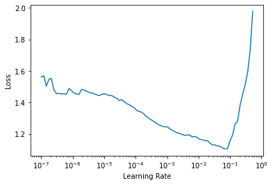
Once everything has been setup, we can find a good learning rate to train the model.
learn.lr_find()
c:\users\wilso\appdata\local\programs\python\python38\lib\site-packages\torch\cuda\nccl.py:14: UserWarning: PyTorch is not compiled with NCCL support
  warnings.warn('PyTorch is not compiled with NCCL support')


SuggestedLRs(lr_min=0.006918309628963471, lr_steep=9.120108734350652e-05)
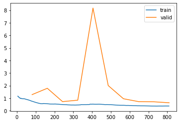
Here we’ll train the model for 10 epochs with one-cycle policy, add a 0.1 weight decay.
learn.fit_one_cycle(10, 6e-3, wd=0.1, cbs=SaveModelCallback(fname='best-val-loss'))
learn.save('efficientnetb3a-1')
| epoch | train_loss | valid_loss | accuracy | time |
|---|---|---|---|---|
| 0 | 0.762553 | 1.285270 | 0.500000 | 02:28 |
| 1 | 0.560403 | 1.788918 | 0.500000 | 02:27 |
| 2 | 0.497399 | 0.727971 | 0.562500 | 02:26 |
| 3 | 0.460750 | 0.842557 | 0.625000 | 02:25 |
| 4 | 0.532170 | 8.171339 | 0.625000 | 02:25 |
| 5 | 0.493482 | 2.005133 | 0.687500 | 02:30 |
| 6 | 0.435214 | 0.956962 | 0.562500 | 03:33 |
| 7 | 0.397469 | 0.727003 | 0.562500 | 03:12 |
| 8 | 0.377309 | 0.713967 | 0.625000 | 02:27 |
| 9 | 0.380401 | 0.636497 | 0.625000 | 02:25 |
Better model found at epoch 0 with valid_loss value: 1.2852699756622314.
Better model found at epoch 2 with valid_loss value: 0.7279710173606873.
Better model found at epoch 7 with valid_loss value: 0.7270027995109558.
Better model found at epoch 8 with valid_loss value: 0.7139670252799988.
Better model found at epoch 9 with valid_loss value: 0.6364966630935669.


Path('models/efficientnetb3a-1.pth')
learn.recorder.plot_loss()
Testing Model
As mentioned, the validation dataset is too small to measure our model’s performance. Fortunately, the dataset gave a large enough test dataset which we’ll be using.
Load Test Data
The method I’ll be using here and for the rest of this notebook is a patchy solution. Specifically, I’ll create a test dataloader and replace the old validation dataset with it.
def get_test_dls(bs, size, test_folder):
    dblock = DataBlock(blocks     = (ImageBlock, CategoryBlock),
                       get_items  = get_image_files,
                       get_y      = parent_label,
                       splitter   = GrandparentSplitter(valid_name=test_folder),
                       item_tfms  = Resize(size),
                       batch_tfms = batch_tfms)
    return dblock.dataloaders(path, bs=bs, num_workers=0).cuda()
test_dl = get_test_dls(64, 224, 'test')
learn.dls = test_dl
Test Accuracy
preds, targs = learn.get_preds()
accuracy(preds, targs)
tensor(0.9231)
Analyze Results
The model achieved a 92% accuracy for the test data. However, using accuracy as a measure of performance in an unbalanced dataset is unwise. If say we have 95 normal chest images and 5 pneumonia-infected ones, freely guessing 100 of them to be normal would still output a high 95% accuracy. Hence, Precision and Recall is a better metric to use in this case.
According to the Scikit Learn docs, precision is intuitively the ability of the classifier not to label as positive a sample that is negative. Whereas recall is intuitively the ability of the classifier to find all the positive samples.
We can plot the results of the test predictions and visualize using a confusion matrix. In fact, plotting such diagram is available in the fast.ai library. However, for some reason I couldn’t get it to work in this new update. Thus, I decided to simply copy the actual fast.ai interpret code and modify it to fix the issue.
I found that the confusion_matrix code broke the plotting process which is dependent on it. To fix the issue, I’ve replaced the confusion matrix with Scitkit Learn’s. Lastly, I specified the function to also print the recall and precision metrics, both of which are from Scikit Learn.
def plot_confusion_matrix(y_pred, y_true, vocab):
    y_pred = y_pred.argmax(dim=-1)
    cm = confusion_matrix(y_true, y_pred)

    fig = plt.figure(figsize=(8,8), dpi=60)
    plt.imshow(cm, interpolation='nearest', cmap="Blues")
    plt.title("Confusion Matrix")
    tick_marks = np.arange(len(vocab))
    plt.xticks(tick_marks, vocab, rotation=90)
    plt.yticks(tick_marks, vocab, rotation=0)

    thresh = cm.max() / 2.
    for i, j in itertools.product(range(cm.shape[0]), range(cm.shape[1])):
        coeff = f'{cm[i, j]}'
        plt.text(j, i, coeff, horizontalalignment="center", verticalalignment="center", color="white" if cm[i, j] > thresh else "black")

    ax = fig.gca()
    ax.set_ylim(len(vocab)-.5,-.5)

    plt.tight_layout()
    plt.ylabel('Actual')
    plt.xlabel('Predicted')
    plt.grid(False)

    print(f"Precision: {precision_score(y_true, y_pred):.3f}")
    print(f"Recall: {recall_score(y_true, y_pred):.3f}")
plot_confusion_matrix(preds, targs, dls.vocab)
Precision: 0.896
Recall: 0.992
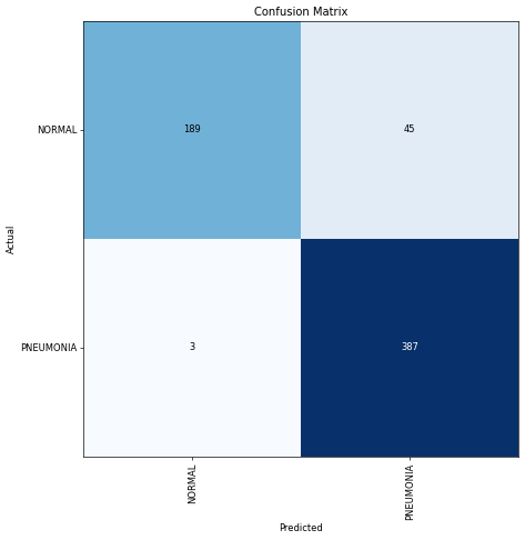
The model achieved 89% precision and 99% recall!
Closing Remarks
Despite all of the issues and troubles I’ve stumbled upon during the project, I’ve learned to be more flexible in utilizing the tools available. I’ve also attempted this task over a year ago as a beginner in deep learning. To my surprise, I’ve actually solved it previously using a VGG19 pretrained model in Tensorflow/Keras and attained quite a satisfying result as well.
In any case, this mini project taught me tons and am excited to learn even more deep learning related topics. Hope you’ve learned something!