MNIST Classification with Quantum Neural Network
Published:
Tensorflow is one of the most used deep learning frameworks today, bundled with many features for end-to-end deep learning processes. Recently, they have just announced a new library on top of Tensorflow, called Tensorflow Quantum. Tensorflow Quantum integrates with Cirq, which provides quantum computing algorithms, and the two works well to do tasks involving Quantum Machine Learning.
Quantum Computer Simulator
Tensorflow Quantum provides a default backend Simulator which is written in C++. It is possible, although slower, to run the backend with a Cirq Simulator, or any other backends like a real quantum computer. However, since real quantum computers of today are still very much noisy and sensitive to inference, the QNN is ran on the C++ simulator backend for simplicity. The aim is to experiment with available hybrid quantum-classical algorithms and see the potential of Quantum Machine Learning once fault-tolerant Quantum Computers become available.
Quantum Neural Networks
One of the realization of Quantum Machine Learning is the implementation of a Quantum Neural Network (QNN), which unlike Hybrid Neural Networks discussed in the previous blog, is purely ran on a quantum circuit with only quantum gates. It does not combines both classical and quantum neural network layers, and works quite differently from how a classical neural network does - at least for now.
MNIST Classification
Again, we’ll be classifying images from the MNIST dataset with the QNN. The following blocks of code were based on a tutorial from Tensorflow Quantum, called MNIST classification. The algorithm used is based on a paper by Farhi et al., and is a must-see paper to see the concepts and the why’s of the QNN being implemented.
Code
Loading Data
Rescaling Images
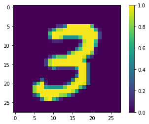
As mentioned, we’ll be using the MNIST dataset as usual, which is originally 28x28 pixels each. We’ll be rescaling the images from $[0, 255]$ to $[0.0, 1.0]$ range.
(x_train, y_train), (x_test, y_test) = tf.keras.datasets.mnist.load_data()
x_train, x_test = x_train[..., np.newaxis]/255.0, x_test[..., np.newaxis]/255.0

print("Number of original training examples:", len(x_train))
print("Number of original test examples:", len(x_test))
Downloading data from https://storage.googleapis.com/tensorflow/tf-keras-datasets/mnist.npz
11493376/11490434 [==============================] - 0s 0us/step
Number of original training examples: 60000
Number of original test examples: 10000
Since the final “output layer” or the readout qubit in this case is only 1, we will only classify 2 distinct classes: 3s and 6s.
def filter_36(x, y):
    keep = (y == 3) | (y == 6)
    x, y = x[keep], y[keep]
    y = y == 3
    return x,y
x_train, y_train = filter_36(x_train, y_train)
x_test, y_test = filter_36(x_test, y_test)

print("Number of filtered training examples:", len(x_train))
print("Number of filtered test examples:", len(x_test))
Number of filtered training examples: 12049
Number of filtered test examples: 1968
print(y_train[0])

plt.imshow(x_train[0, :, :, 0])
plt.colorbar()
True


<matplotlib.colorbar.Colorbar at 0x7f453da67898>
Downsampling Images
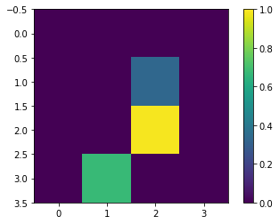
The images are then downsampled to 4x4 pixels each since we’ll only be using 17 qubits, 16 for the images, and 1 as the readout. This does lower down the resolution of the original image to the point of not representing how it looks originally. But due to the limitation of number of qubits simulatable, downsampling to low resolution images is required.
x_train_small = tf.image.resize(x_train, (4,4)).numpy()
x_test_small = tf.image.resize(x_test, (4,4)).numpy()
print(y_train[0])

plt.imshow(x_train_small[0,:,:,0], vmin=0, vmax=1)
plt.colorbar()
True


<matplotlib.colorbar.Colorbar at 0x7f453022d7b8>
Removing Contradicting Images
Additionally, there are ambiguous labels in our dataset whereby 1 image has more than 1 labels. We’ll remove those contradicting image-label pairs from the dataset.
def remove_contradicting(xs, ys):
    mapping = collections.defaultdict(set)
    for x,y in zip(xs,ys):
       mapping[tuple(x.flatten())].add(y)

    new_x = []
    new_y = []
    for x,y in zip(xs, ys):
      labels = mapping[tuple(x.flatten())]
      if len(labels) == 1:
          new_x.append(x)
          new_y.append(list(labels)[0])
      else:
          pass

    num_3 = sum(1 for value in mapping.values() if True in value)
    num_6 = sum(1 for value in mapping.values() if False in value)
    num_both = sum(1 for value in mapping.values() if len(value) == 2)

    print("Number of unique images:", len(mapping.values()))
    print("Number of 3s: ", num_3)
    print("Number of 6s: ", num_6)
    print("Number of contradictory images: ", num_both)
    print()
    print("Initial number of examples: ", len(xs))
    print("Remaining non-contradictory examples: ", len(new_x))

    return np.array(new_x), np.array(new_y)
x_train_nocon, y_train_nocon = remove_contradicting(x_train_small, y_train)
Number of unique images: 10387
Number of 3s:  4961
Number of 6s:  5475
Number of contradictory images:  49

Initial number of examples:  12049
Remaining non-contradictory examples:  11520
Encoding Data as Quantum Circuits
We have to find a way to represent our images as qubits, and the method implemented in the tutorial is pretty straightforward. We set a certain threshold value, in our case 0.5, and if our pixel value is greater than that, we’ll append Cirq’s X-gate, which flips the qubit state from a $0$ to a $1$ (i.e. signifying the existence of a pixel value in a qubit).
THRESHOLD = 0.5

x_train_bin = np.array(x_train_nocon > THRESHOLD, dtype=np.float32)
x_test_bin = np.array(x_test_small > THRESHOLD, dtype=np.float32)
def convert_to_circuit(image):
    """Encode truncated classical image into quantum datapoint."""
    values = np.ndarray.flatten(image)
    qubits = cirq.GridQubit.rect(4, 4)
    circuit = cirq.Circuit()
    for i, value in enumerate(values):
        if value:
            circuit.append(cirq.X(qubits[i]))
    return circuit


x_train_circ = [convert_to_circuit(x) for x in x_train_bin]
x_test_circ = [convert_to_circuit(x) for x in x_test_bin]
Let’s see how one of our training data now looks like once encoded into a circuit. Do note that qubits without operations aren’t printed out.
SVGCircuit(x_train_circ[0])

Lastly, in order to enable the usage of the newly created datapoint, we have to convert it from a circuit back into a tensor.
x_train_tfcirc = tfq.convert_to_tensor(x_train_circ)
x_test_tfcirc = tfq.convert_to_tensor(x_test_circ)
Quantum Neural Network
Now that we have encoded our data that is able to flow through a Tensorflow Quantum’s layers, we’ll begin to create our model. The type of QNN which is implemented in the paper utilizes two-qubit gates that connects every data qubit in the circuit to the readout qubit. At the end of the circuit, the expectation of the readout qubit will then be measured as the basis of our model’s classification.
Building Circuit Layers
Each layer uses $n$ instances of the same gate, with each of the data qubits acting on the readout qubit. The following class adds a layer of that gate to the circuit.
class CircuitLayerBuilder():
    def __init__(self, data_qubits, readout):
        self.data_qubits = data_qubits
        self.readout = readout

    def add_layer(self, circuit, gate, prefix):
        for i, qubit in enumerate(self.data_qubits):
            symbol = sympy.Symbol(prefix + '-' + str(i))
            circuit.append(gate(qubit, self.readout)**symbol)
Let’s see how it would look like in a sample circuit.
demo_builder = CircuitLayerBuilder(data_qubits = cirq.GridQubit.rect(4,1),
                                   readout=cirq.GridQubit(-1,-1))

circuit = cirq.Circuit()
demo_builder.add_layer(circuit, gate = cirq.XX, prefix='xx')
SVGCircuit(circuit)

As you can see, all data qubits (4 in this case) are connected with the readout qubit via an Ising ($XX$) Coupling gate.
Creating Quantum Model
With the quantum layer class ready for use, we can create the quantum model for our QNN. Instead of only using a single Ising ($XX$) Coupling Gate, we’ll also add Ising ($ZZ$) Coupling Gate for every data qubit. These gates have their respective parameters, which our model will learn to optimize later on.
Notice that we’re adding two intial gates to the readout qubit, an $X$ gate to convert it into the state $1$, and an $H$ to set our qubit in superposition. After all the Ising Coupling gates, we’ll finally append another $H$ gate to our readout qubit to bring it out of superposition, before finally doing a $Z$-measurement to obtain the expectation value.
def create_quantum_model():
    data_qubits = cirq.GridQubit.rect(4, 4)  # a 4x4 grid.
    readout = cirq.GridQubit(-1, -1)         # a single qubit at [-1,-1]
    circuit = cirq.Circuit()

    # Prepare the readout qubit.
    circuit.append(cirq.X(readout))
    circuit.append(cirq.H(readout))

    builder = CircuitLayerBuilder(
        data_qubits = data_qubits,
        readout=readout)

    # Then add layers (experiment by adding more).
    builder.add_layer(circuit, cirq.XX, "xx1")
    builder.add_layer(circuit, cirq.ZZ, "zz1")

    # Finally, prepare the readout qubit.
    circuit.append(cirq.H(readout))

    return circuit, cirq.Z(readout)
model_circuit, model_readout = create_quantum_model()
The model’s pretty huge since it has 17 qubits in total, and if we try to see how it looks when laid out on a flat circuit, it looks like the following:
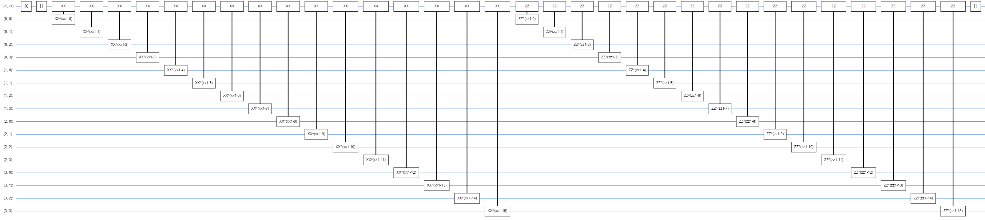
Wrapping Model-Circuit in TF-Quantum Model
To bring all things we’ve built together, Tensorflow Quantum model/circuit interfaces with the normal Keras Sequential model. We’ll prepend an input layer which takes the encoded data from earlier, before finally feeding it into the quantum circuit. Since the parameters of the quantum circuits are the one we would like the model to learn upon, we’ll wrap it with the tfq.layers.PQC layer which returns the expectation value of the readout qubit.
model = tf.keras.Sequential([
    tf.keras.layers.Input(shape=(), dtype=tf.string),
    tfq.layers.PQC(model_circuit, model_readout),
])
The PQC layer will return its results within the range $[-1, 1]$, and using the hinge-loss is suitable although it requires us encoding the target labels like the following:
y_train_hinge = 2.0*y_train_nocon-1.0
y_test_hinge = 2.0*y_test-1.0
It should be noted that we could instead shift the model’s output range to $[0, 1]$ and treat it as the probability the model assigns to class 3 to be used with the usual tf.losses.BinaryCrossentropy loss function.
We then specify a hinge accuracy metric which handles $[-1, 1]$ as the target labels argument.
def hinge_accuracy(y_true, y_pred):
    y_true = tf.squeeze(y_true) > 0.0
    y_pred = tf.squeeze(y_pred) > 0.0
    result = tf.cast(y_true == y_pred, tf.float32)

    return tf.reduce_mean(result)
Lastly, we’ll do the usual model.compile(), passing it our loss function, optimizer, and the metrics to be recorded.
model.compile(
    loss=tf.keras.losses.Hinge(),
    optimizer=tf.keras.optimizers.Adam(),
    metrics=[hinge_accuracy])
print(model.summary())
Model: "sequential"
_________________________________________________________________
Layer (type)                 Output Shape              Param #
=================================================================
pqc (PQC)                    (None, 1)                 32
=================================================================
Total params: 32
Trainable params: 32
Non-trainable params: 0
_________________________________________________________________
None
Training Quantum Neural Network
With everything in place and ready for training, we’ll begin the training of our model. Luckily, Tensorflow Quantum provides a default Differentiator which handles backpropagation through the quantum circuit, so we do not need to handle that manually. It is possible however, to provide it with our own Differentiator function, but we won’t be doing that here.
We’ll first decide the number of epochs, batch size, and the number of examples to be used for training. As there are quite many training images, we can always use a subset of it just to decrease training duration and to just see the model learn.
EPOCHS = 3
BATCH_SIZE = 32

NUM_EXAMPLES = 500
x_train_tfcirc_sub = x_train_tfcirc[:NUM_EXAMPLES]
y_train_hinge_sub = y_train_hinge[:NUM_EXAMPLES]
qnn_history = model.fit(
      x_train_tfcirc_sub, y_train_hinge_sub,
      batch_size=32,
      epochs=EPOCHS,
      verbose=1,
      validation_data=(x_test_tfcirc, y_test_hinge))

qnn_results = model.evaluate(x_test_tfcirc, y_test)
Train on 500 samples, validate on 1968 samples
Epoch 1/3
500/500 [==============================] - 301s 602ms/sample - loss: 0.9929 - hinge_accuracy: 0.6199 - val_loss: 0.9887 - val_hinge_accuracy: 0.6739
Epoch 2/3
500/500 [==============================] - 300s 600ms/sample - loss: 0.9849 - hinge_accuracy: 0.6777 - val_loss: 0.9808 - val_hinge_accuracy: 0.6774
Epoch 3/3
500/500 [==============================] - 301s 602ms/sample - loss: 0.9756 - hinge_accuracy: 0.6746 - val_loss: 0.9687 - val_hinge_accuracy: 0.6809
1968/1968 [==============================] - 34s 17ms/sample - loss: 0.9687 - hinge_accuracy: 0.6809
Note that the training accuracy reports the average over the epoch. While the validation accuracy is evaluated at the end of each epoch. Here, our model obtained about 0.68 validation hinge accuracy, and just like any other quantum or hybrid neural networks, this value varies from trials to trials. The highest accuracy I have obtained with the same exact subdataset and circuit was 0.80.
Classical Neural Network
A classical neural network will definitely outperform this QNN, even if we use a very simple classical Convolutional Neural Network (CNN). The tutorial showed an example of a CNN based off LeNet from a Keras tutorial.
def create_classical_model():
    model = tf.keras.Sequential()
    model.add(tf.keras.layers.Conv2D(32, [3, 3], activation='relu', input_shape=(28,28,1)))
    model.add(tf.keras.layers.Conv2D(64, [3, 3], activation='relu'))
    model.add(tf.keras.layers.MaxPooling2D(pool_size=(2, 2)))
    model.add(tf.keras.layers.Dropout(0.25))
    model.add(tf.keras.layers.Flatten())
    model.add(tf.keras.layers.Dense(128, activation='relu'))
    model.add(tf.keras.layers.Dropout(0.5))
    model.add(tf.keras.layers.Dense(1))
    return model


model = create_classical_model()
model.compile(loss=tf.keras.losses.BinaryCrossentropy(from_logits=True),
              optimizer=tf.keras.optimizers.Adam(),
              metrics=['accuracy'])

model.summary()
Model: "sequential_1"
_________________________________________________________________
Layer (type)                 Output Shape              Param #
=================================================================
conv2d (Conv2D)              (None, 26, 26, 32)        320
_________________________________________________________________
conv2d_1 (Conv2D)            (None, 24, 24, 64)        18496
_________________________________________________________________
max_pooling2d (MaxPooling2D) (None, 12, 12, 64)        0
_________________________________________________________________
dropout (Dropout)            (None, 12, 12, 64)        0
_________________________________________________________________
flatten (Flatten)            (None, 9216)              0
_________________________________________________________________
dense (Dense)                (None, 128)               1179776
_________________________________________________________________
dropout_1 (Dropout)          (None, 128)               0
_________________________________________________________________
dense_1 (Dense)              (None, 1)                 129
=================================================================
Total params: 1,198,721
Trainable params: 1,198,721
Non-trainable params: 0
_________________________________________________________________
model.fit(x_train,
          y_train,
          batch_size=128,
          epochs=1,
          verbose=1,
          validation_data=(x_test, y_test))

cnn_results = model.evaluate(x_test, y_test)
Train on 12049 samples, validate on 1968 samples
12049/12049 [==============================] - 7s 557us/sample - loss: 0.0397 - accuracy: 0.9854 - val_loss: 0.0053 - val_accuracy: 0.9990
1968/1968 [==============================] - 0s 144us/sample - loss: 0.0053 - accuracy: 0.9990
In just a single epoch, the classical CNN was able to achieve 0.99 validation accuracy. Although it looks like a simple CNN, it does however, get fed by the original 28x28 pixels image and has 1.2M parameters. Hence it’s not really fair to compare it to our QNN.
To put them into a fair level, we’ll create a 37-parameter classical neural network which also resizes the images to 4x4 pixels each.
def create_fair_classical_model():
    model = tf.keras.Sequential()
    model.add(tf.keras.layers.Flatten(input_shape=(4,4,1)))
    model.add(tf.keras.layers.Dense(2, activation='relu'))
    model.add(tf.keras.layers.Dense(1))
    return model


model = create_fair_classical_model()
model.compile(loss=tf.keras.losses.BinaryCrossentropy(from_logits=True),
              optimizer=tf.keras.optimizers.Adam(),
              metrics=['accuracy'])

model.summary()
Model: "sequential_2"
_________________________________________________________________
Layer (type)                 Output Shape              Param #
=================================================================
flatten_1 (Flatten)          (None, 16)                0
_________________________________________________________________
dense_2 (Dense)              (None, 2)                 34
_________________________________________________________________
dense_3 (Dense)              (None, 1)                 3
=================================================================
Total params: 37
Trainable params: 37
Non-trainable params: 0
_________________________________________________________________
model.fit(x_train_bin,
          y_train_nocon,
          batch_size=128,
          epochs=20,
          verbose=2,
          validation_data=(x_test_bin, y_test))

fair_nn_results = model.evaluate(x_test_bin, y_test)
Train on 11520 samples, validate on 1968 samples
Epoch 1/20
11520/11520 - 1s - loss: 0.7959 - accuracy: 0.4551 - val_loss: 0.7675 - val_accuracy: 0.4853
Epoch 2/20
11520/11520 - 0s - loss: 0.7290 - accuracy: 0.5030 - val_loss: 0.7130 - val_accuracy: 0.4868
Epoch 3/20
11520/11520 - 0s - loss: 0.6995 - accuracy: 0.5031 - val_loss: 0.6968 - val_accuracy: 0.4868
Epoch 4/20
11520/11520 - 0s - loss: 0.6918 - accuracy: 0.5034 - val_loss: 0.6925 - val_accuracy: 0.4878
Epoch 5/20
11520/11520 - 0s - loss: 0.6847 - accuracy: 0.5103 - val_loss: 0.6793 - val_accuracy: 0.4924
Epoch 6/20
11520/11520 - 0s - loss: 0.6553 - accuracy: 0.5845 - val_loss: 0.6425 - val_accuracy: 0.6316
Epoch 7/20
11520/11520 - 0s - loss: 0.5934 - accuracy: 0.6980 - val_loss: 0.5676 - val_accuracy: 0.7429
Epoch 8/20
11520/11520 - 0s - loss: 0.5298 - accuracy: 0.8106 - val_loss: 0.5105 - val_accuracy: 0.8216
Epoch 9/20
11520/11520 - 0s - loss: 0.4782 - accuracy: 0.8536 - val_loss: 0.4658 - val_accuracy: 0.8323
Epoch 10/20
11520/11520 - 0s - loss: 0.4386 - accuracy: 0.8595 - val_loss: 0.4318 - val_accuracy: 0.8333
Epoch 11/20
11520/11520 - 0s - loss: 0.4068 - accuracy: 0.8617 - val_loss: 0.4039 - val_accuracy: 0.8338
Epoch 12/20
11520/11520 - 0s - loss: 0.3811 - accuracy: 0.8635 - val_loss: 0.3813 - val_accuracy: 0.8338
Epoch 13/20
11520/11520 - 0s - loss: 0.3599 - accuracy: 0.8641 - val_loss: 0.3624 - val_accuracy: 0.8328
Epoch 14/20
11520/11520 - 0s - loss: 0.3421 - accuracy: 0.8648 - val_loss: 0.3465 - val_accuracy: 0.8328
Epoch 15/20
11520/11520 - 0s - loss: 0.3270 - accuracy: 0.8720 - val_loss: 0.3329 - val_accuracy: 0.8714
Epoch 16/20
11520/11520 - 0s - loss: 0.3140 - accuracy: 0.8874 - val_loss: 0.3210 - val_accuracy: 0.8714
Epoch 17/20
11520/11520 - 0s - loss: 0.3028 - accuracy: 0.8876 - val_loss: 0.3109 - val_accuracy: 0.8714
Epoch 18/20
11520/11520 - 0s - loss: 0.2931 - accuracy: 0.8876 - val_loss: 0.3019 - val_accuracy: 0.8714
Epoch 19/20
11520/11520 - 0s - loss: 0.2846 - accuracy: 0.8876 - val_loss: 0.2941 - val_accuracy: 0.8714
Epoch 20/20
11520/11520 - 0s - loss: 0.2771 - accuracy: 0.8873 - val_loss: 0.2872 - val_accuracy: 0.8714
1968/1968 [==============================] - 0s 78us/sample - loss: 0.2872 - accuracy: 0.8714
Unsurprisingly, the model performed better and arguably more stable than the QNN for obvious reasons. The data is very much classical, so its reasonable why a classical neural network would outperform a quantum one.
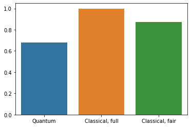
qnn_accuracy = qnn_results[1]
cnn_accuracy = cnn_results[1]
fair_nn_accuracy = fair_nn_results[1]

sns.barplot(["Quantum", "Classical, full", "Classical, fair"],
            [qnn_accuracy, cnn_accuracy, fair_nn_accuracy])
<matplotlib.axes._subplots.AxesSubplot at 0x7f44e28fd518>
Experiments
After learning how to create a QNN from the tutorial, I decided to play around with the number of parameters in the model. Instead of using only 1 Ising $(XX)$ Coupling Gate and 1 Ising $(ZZ)$ Coupling Gate, I’ve decided to use 2 of each kinds, which adds additional 32 parameters to the model, summing to 64 parameters in total.
def create_quantum_model():
    data_qubits = cirq.GridQubit.rect(4, 4)
    readout = cirq.GridQubit(-1, -1)
    circuit = cirq.Circuit()

    circuit.append(cirq.X(readout))
    circuit.append(cirq.H(readout))

    builder = CircuitLayerBuilder(
        data_qubits = data_qubits,
        readout=readout)

    builder.add_layer(circuit, cirq.XX, "xx1")
    builder.add_layer(circuit, cirq.XX, "xx2")
    builder.add_layer(circuit, cirq.ZZ, "zz1")
    builder.add_layer(circuit, cirq.ZZ, "zz2")

    circuit.append(cirq.H(readout))

    return circuit, cirq.Z(readout)
print(model.summary())
Model: "sequential"
_________________________________________________________________
Layer (type)                 Output Shape              Param #
=================================================================
pqc (PQC)                    (None, 1)                 64
=================================================================
Total params: 64
Trainable params: 64
Non-trainable params: 0
_________________________________________________________________
None
I have also used a total of 1000 sample images instead of only 500, just for fun. The rest are kept identical.
EPOCHS = 3
BATCH_SIZE = 32

NUM_EXAMPLES = 1000
qnn_history = model.fit(
      x_train_tfcirc_sub, y_train_hinge_sub,
      batch_size=32,
      epochs=EPOCHS,
      verbose=1,
      validation_data=(x_test_tfcirc, y_test_hinge))

qnn_results = model.evaluate(x_test_tfcirc, y_test)
Train on 1000 samples, validate on 1968 samples
Epoch 1/3
1000/1000 [==============================] - 1693s 2s/sample - loss: 0.9964 - hinge_accuracy: 0.6748 - val_loss: 0.9851 - val_hinge_accuracy: 0.7999
Epoch 2/3
1000/1000 [==============================] - 1704s 2s/sample - loss: 0.9271 - hinge_accuracy: 0.8066 - val_loss: 0.8194 - val_hinge_accuracy: 0.7964
Epoch 3/3
1000/1000 [==============================] - 1593s 2s/sample - loss: 0.6629 - hinge_accuracy: 0.7988 - val_loss: 0.5120 - val_hinge_accuracy: 0.7964
1968/1968 [==============================] - 50s 25ms/sample - loss: 0.5120 - hinge_accuracy: 0.7964
As you can see, the validation hinge accuracy this time is about 0.79 and a much lower validation loss, which is better than our 32-parameter model previously. It should be noted again that these values change from trials to trials, so a 1-time attempt do not represent the model’s performance entirely.
Closing Remarks
Issues with Quantum Neural Network
As discussed in the previous post, there are still issues regarding QNNs and Quantum Computers in general. There are no analytical way to get the gradients of the quantum layers yet, and sometimes the circuit’s gradient vanishes as the model learns. There’s definitely a huge area of possible improvements as well as research to the possibilities of Quantum Neural Network in tackling the limits of a classical neural network.
Conclusion
It’s been a ride learning how the Quantum Neural Network was implemented. It is very much different from how a classical neural network is implemented, and there are many factors to consider since the capabilities of a Quantum Computer and its simulators are still limited. However, it was still a mind-blowing experience to take a glimpse of the future potential of Quantum Computers and what it can offer to the Machine Learning domain.
Credits
Portions of this page are modifications based on work created and shared by Google and used according to terms described in the Creative Commons 4.0 Attribution License.