
MNIST Classification with Hybrid Quantum-Classical Neural Network
Published:
Qiskit is IBM’s open-source framework to do quantum processes which provides users access to both simulators and real Quantum Computers. Today, the Quantum Computer available is still in the Noisy Intermediate-Scale Quantum (NISQ) era and is very much sensitive to any forms of interference. Unlike real Quantum Computers, simulators provided by Qiskit aren’t noisy and is great for prototyping.
Hybrid Quantum-Classical Neural Network
Qiskit and PyTorch provides a way to connect classical neural networks with quantum circuit, thus creating a hybrid quantum-classical NN. A tutorial is provided under the Qiskit textbook, and will be the basis of the code shown in this post.
Forward Pass
How a hybrid NN works in forward pass is shown in the following diagram:
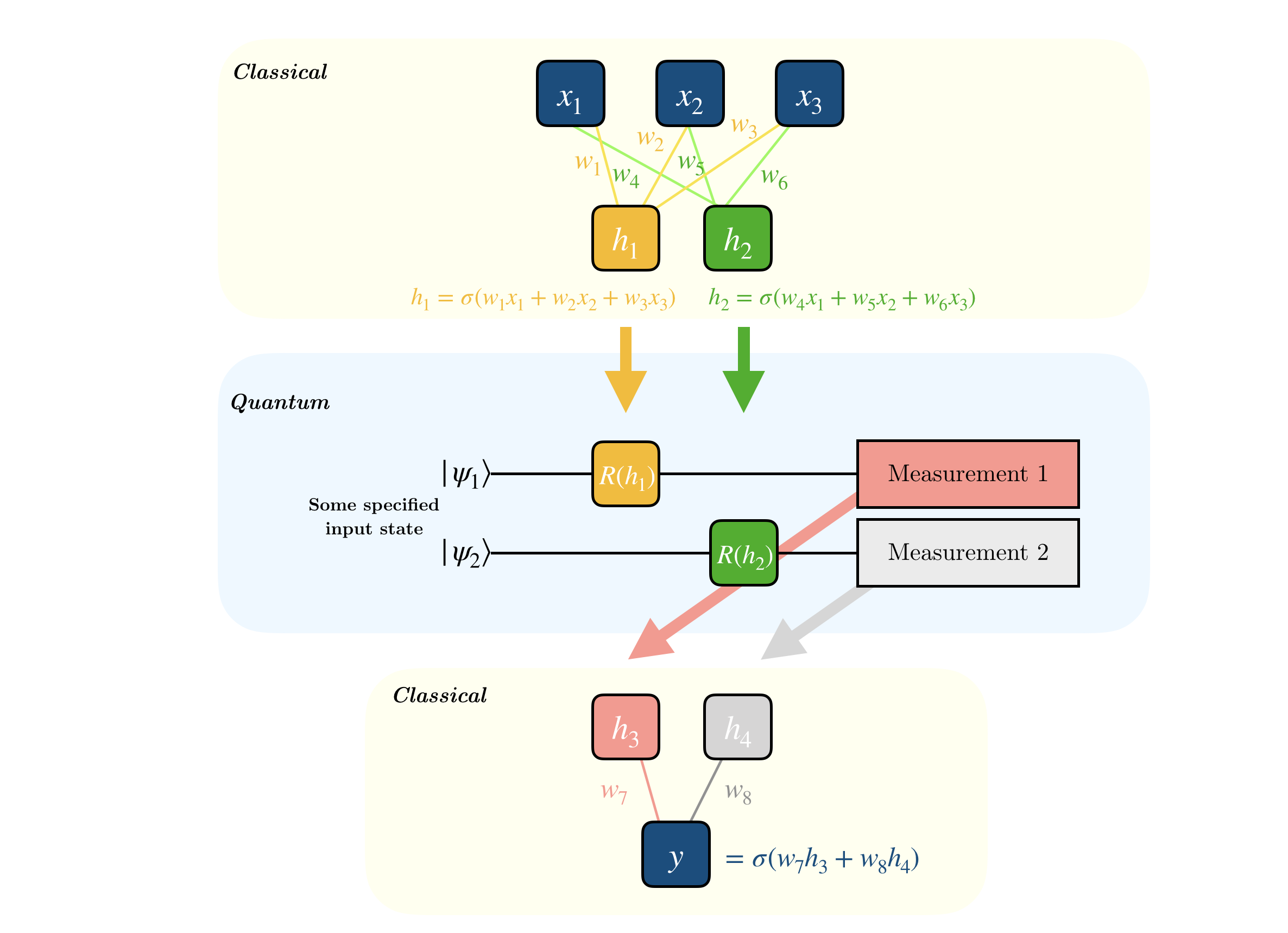
As shown above, the neural network will have its usual classical layers at the start, a quantum “layer” in between, and followed by classical layers again. It is the parameters of the quantum layer which the neural network will learn to optimize.
The layers used in the classical part is arbitrary, however it should be noted that the output of the classical layers at the start should conform to the input of the quantum layer (which we’ll see later in code). Similarly, the output of the quantum layer should be in-line with the input of the following classical layer.
Backward Pass
This raises a question especially during the backpropagation process. The derivative of the quantum layer is required to perform gradient descent - a critical step to optimizing the model. To tackle the problem, we’ll be using the parameter shift rule to find its gradient, which is calculated as follows:

The parameter shift rule is parallel to how finite difference works: making a small shift and calculating the change in the output with respect to the small shift. Details won’t be discussed here.
MNIST Classification
MNIST is a go-to dataset for image classification as it is simple for a beginner. Similarly, we’ll be using MNIST to test out how our hybrid NN performs. In this case however, we’ll be only classifying 2 digits instead of the usual 10.
Code: Classifying 0s and 1s
Quantum Circuit
As mentioned above, we’ll create a quantum circuit whose parameter we’ll let the neural network tweak as it learns. The example given in the textbook is a very simple, 1-qubit circuit with two gates, a Hadamard and a $RY$ gate. A $RY$ rotation has a parameter called $\theta$ which is precisely the parameter to be optimized.
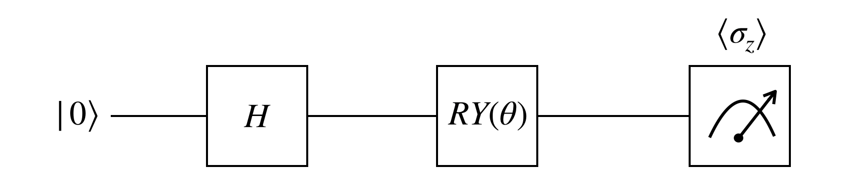
After going the two gates, the qubit is then measured. It is the result of this measurement which we’ll use as the final output of the neural network. A 1-qubit measurement has only two possible outputs, and the two possible outputs in our case corresponds to the two possible classes which an image belong to. To measure the $z$-basis output, we’ll be calculating the $\sigma_z$ expected value the same way as we would calculate expected value in statistics.
\[\sigma_z = \sum_{i} z_i \cdot p(z_i)\]Later, we’ll specify the circuit how many shots or trials we’d like to make.
Let’s implement the circuit in Qiskit!
class QuantumCircuit:
    def __init__(self, n_qubits, backend, shots):
        # --- Circuit definition ---
        self._circuit = qiskit.QuantumCircuit(n_qubits)

        all_qubits = [i for i in range(n_qubits)]
        self.theta = qiskit.circuit.Parameter('theta')

        self._circuit.h(all_qubits)
        self._circuit.barrier()
        self._circuit.ry(self.theta, all_qubits)

        self._circuit.measure_all()
        # ---------------------------

        self.backend = backend
        self.shots = shots

    def run(self, thetas):
        job = qiskit.execute(self._circuit,
                             self.backend,
                             shots = self.shots,
                             parameter_binds = [{self.theta: theta} for theta in thetas])
        result = job.result().get_counts(self._circuit)

        counts = np.array(list(result.values()))
        states = np.array(list(result.keys())).astype(float)

        # Compute probabilities for each state
        probabilities = counts / self.shots
        # Get state expectation
        expectation = np.sum(states * probabilities)

        return np.array([expectation])
Testing Quantum Circuit
Just for fun, the textbook gave a test implementation of the circuit if we were to run it as usual. We’ll specify that we’ll need 1 qubit, provide the simulator to be used, give it 100 shots and use $\pi$ as our angle.
simulator = qiskit.Aer.get_backend('qasm_simulator')
circuit = QuantumCircuit(1, simulator, 100)
print('Expected value for rotation pi: {}'.format(circuit.run([np.pi])[0]))
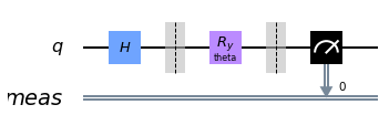
circuit._circuit.draw(output='mpl')
Expected value for rotation pi: 0.5
Quantum-Classical Class
After creating the designated circuit, we can utilize it to create a hybrid class/layer with PyTorch. We specify the forward pass to be pretty much running the circuit, and the backward pass to be the parameter shift rule we discussed earlier.
class HybridFunction(Function):
    @staticmethod
    def forward(ctx, input, quantum_circuit, shift):
        """ Forward pass computation """
        ctx.shift = shift
        ctx.quantum_circuit = quantum_circuit

        expectation_z = ctx.quantum_circuit.run(input[0].tolist())
        result = torch.tensor([expectation_z])
        ctx.save_for_backward(input, result)

        return result

    @staticmethod
    def backward(ctx, grad_output):
        """ Backward pass computation """
        input, expectation_z = ctx.saved_tensors
        input_list = np.array(input.tolist())

        shift_right = input_list + np.ones(input_list.shape) * ctx.shift
        shift_left = input_list - np.ones(input_list.shape) * ctx.shift

        gradients = []
        for i in range(len(input_list)):
            expectation_right = ctx.quantum_circuit.run(shift_right[i])
            expectation_left  = ctx.quantum_circuit.run(shift_left[i])

            gradient = torch.tensor([expectation_right]) - torch.tensor([expectation_left])
            gradients.append(gradient)
        gradients = np.array([gradients]).T
        return torch.tensor([gradients]).float() * grad_output.float(), None, None
With that we can create an actual PyTorch layer which inherits from nn.Module which just applies whatever we’ve implemented in HybridFunction.
class Hybrid(nn.Module):
    def __init__(self, backend, shots, shift):
        super(Hybrid, self).__init__()
        self.quantum_circuit = QuantumCircuit(1, backend, shots)
        self.shift = shift

    def forward(self, input):
        return HybridFunction.apply(input, self.quantum_circuit, self.shift)
Loading Data
Training Dataset
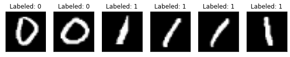
As mentioned, we’ll use MNIST but only two of its classes, specifically 0s and 1s. We’ll load up the dataset from PyTorch datasets for training and testing purposes. Only 100 samples were used for training and 50 for testing in the example.
n_samples = 100

X_train = datasets.MNIST(root='./data', train=True, download=True,
                         transform=transforms.Compose([transforms.ToTensor()]))

# Leaving only labels 0 and 1
idx = np.append(np.where(X_train.targets == 0)[0][:n_samples],
                np.where(X_train.targets == 1)[0][:n_samples])

X_train.data = X_train.data[idx]
X_train.targets = X_train.targets[idx]

train_loader = torch.utils.data.DataLoader(X_train, batch_size=1, shuffle=True)
n_samples_show = 6

data_iter = iter(train_loader)
fig, axes = plt.subplots(nrows=1, ncols=n_samples_show, figsize=(10, 3))

while n_samples_show > 0:
    images, targets = data_iter.__next__()

    axes[n_samples_show - 1].imshow(images[0].numpy().squeeze(), cmap='gray')
    axes[n_samples_show - 1].set_xticks([])
    axes[n_samples_show - 1].set_yticks([])
    axes[n_samples_show - 1].set_title("Labeled: {}".format(targets.item()))

    n_samples_show -= 1
Testing Dataset
n_samples = 50

X_test = datasets.MNIST(root='./data', train=False, download=True,
                        transform=transforms.Compose([transforms.ToTensor()]))

idx = np.append(np.where(X_test.targets == 0)[0][:n_samples],
                np.where(X_test.targets == 1)[0][:n_samples])

X_test.data = X_test.data[idx]
X_test.targets = X_test.targets[idx]

test_loader = torch.utils.data.DataLoader(X_test, batch_size=1, shuffle=True)
Hybrid Neural Network
With most of the things in-place, we can begin to create our model. The classical layers we’ll use are normal convolution, dropout and linear layers. Notice that the final linear layer fc2 only has 1 output since our quantum layer has only 1 parameter. Also, the final output of the forward pass concatenates the two probabilities into one tensor which we’ll later pass to our loss function.
class Net(nn.Module):
    def __init__(self):
        super(Net, self).__init__()
        self.conv1 = nn.Conv2d(1, 32, kernel_size=5)
        self.conv2 = nn.Conv2d(32, 64, kernel_size=5)
        self.dropout = nn.Dropout2d()
        self.fc1 = nn.Linear(256, 64)
        self.fc2 = nn.Linear(64, 1)
        self.hybrid = Hybrid(qiskit.Aer.get_backend('qasm_simulator'), 100, np.pi / 2)

    def forward(self, x):
        x = F.relu(self.conv1(x))
        x = F.relu(self.conv2(x))
        x = F.max_pool2d(x, 2)
        x = self.dropout(x)
        x = x.view(-1, 256)
        x = F.relu(self.fc1(x))
        x = self.fc2(x)
        x = self.hybrid(x)
        return torch.cat((x, 1 - x), -1)
Training Neural Network
Finally, we’ll train our model just as we would train a normal image classification model. We’ve implemented all the backward pass processes in the quantum layer, so doing loss.backward() would correspond to the parameter shift rule previously.
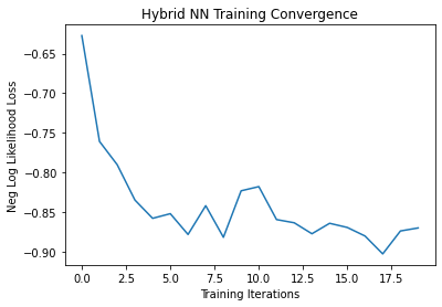
We’ll train for 20 epochs and record the loss after each iteration.
plt.plot(loss_list)
plt.title('Hybrid NN Training Convergence')
plt.xlabel('Training Iterations')
plt.ylabel('Neg Log Likelihood Loss')model = Net()
optimizer = optim.Adam(model.parameters(), lr=0.001)
loss_func = nn.NLLLoss()

epochs = 20
loss_list = []

model.train()
for epoch in range(epochs):
    total_loss = []
    for batch_idx, (data, target) in enumerate(train_loader):
        optimizer.zero_grad()
        # Forward pass
        output = model(data)
        # Calculating loss
        loss = loss_func(output, target)
        # Backward pass
        loss.backward()
        # Optimize the weights
        optimizer.step()

        total_loss.append(loss.item())
    loss_list.append(sum(total_loss)/len(total_loss))
    print('Training [{:.0f}%]\tLoss: {:.4f}'.format(
        100. * (epoch + 1) / epochs, loss_list[-1]))
Training [5%]	Loss: -0.6274
Training [10%]	Loss: -0.7605
Training [15%]	Loss: -0.7898
Training [20%]	Loss: -0.8343
Training [25%]	Loss: -0.8573
Training [30%]	Loss: -0.8514
Training [35%]	Loss: -0.8776
Training [40%]	Loss: -0.8414
Training [45%]	Loss: -0.8811
Training [50%]	Loss: -0.8226
Training [55%]	Loss: -0.8174
Training [60%]	Loss: -0.8588
Training [65%]	Loss: -0.8629
Training [70%]	Loss: -0.8767
Training [75%]	Loss: -0.8635
Training [80%]	Loss: -0.8688
Training [85%]	Loss: -0.8795
Training [90%]	Loss: -0.9021
Training [95%]	Loss: -0.8732
Training [100%]	Loss: -0.8694
plt.plot(loss_list)
plt.title('Hybrid NN Training Convergence')
plt.xlabel('Training Iterations')
plt.ylabel('Neg Log Likelihood Loss')
Text(0, 0.5, 'Neg Log Likelihood Loss')
Testing Neural Network
As seen in the diagram above, our loss has gradually decreased and it seems that the model had learned well. To see how it fairs, let’s test it out with the test data we’ve set apart earlier.
model.eval()
with torch.no_grad():

    correct = 0
    for batch_idx, (data, target) in enumerate(test_loader):
        output = model(data)

        pred = output.argmax(dim=1, keepdim=True)
        correct += pred.eq(target.view_as(pred)).sum().item()

        loss = loss_func(output, target)
        total_loss.append(loss.item())

    print('Performance on test data:\n\tLoss: {:.4f}\n\tAccuracy: {:.1f}%'.format(
        sum(total_loss) / len(total_loss),
        correct / len(test_loader) * 100)
        )
Performance on test data:
	Loss: -0.8713
	Accuracy: 100.0%
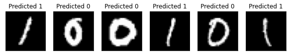
Notice that the model has achieved 100% accuracy with the small test dataset, which is reasonable.
n_samples_show = 6
count = 0
fig, axes = plt.subplots(nrows=1, ncols=n_samples_show, figsize=(10, 3))

model.eval()
with torch.no_grad():
    for batch_idx, (data, target) in enumerate(test_loader):
        if count == n_samples_show:
            break
        output = model(data)

        pred = output.argmax(dim=1, keepdim=True)

        axes[count].imshow(data[0].numpy().squeeze(), cmap='gray')

        axes[count].set_xticks([])
        axes[count].set_yticks([])
        axes[count].set_title('Predicted {}'.format(pred.item()))

        count += 1
Code: Classifying 3s and 7s
With what the model can achieve, I tried to change the dataset used. Instead of using 0s and 1s which look fairly different from each other, I tried to replace them with 3s and 7s to see how the model performs. The processes except the data-loading is pretty much identical.
Loading Data
Training Dataset
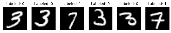
Here we’ll specify that we want 3s and 7s, and encode their labels to 0 and 1 respectively.
n_samples = 100

X_train = datasets.MNIST(root='./data', train=True, download=True,
                         transform=transforms.Compose([transforms.ToTensor()]))

# Leaving only labels 3 and 7
idx = np.append(np.where(X_train.targets == 3)[0][:n_samples],
                np.where(X_train.targets == 7)[0][:n_samples])

X_train.data = X_train.data[idx]
X_train.targets = X_train.targets[idx]
# Encode into 0 and 1
X_train.targets = torch.tensor(list(map(lambda x: 0 if x == 3 else 1, X_train.targets)))

train_loader = torch.utils.data.DataLoader(X_train, batch_size=1, shuffle=True)
n_samples_show = 6

data_iter = iter(train_loader)
fig, axes = plt.subplots(nrows=1, ncols=n_samples_show, figsize=(10, 3))

while n_samples_show > 0:
    images, targets = data_iter.__next__()

    axes[n_samples_show - 1].imshow(images[0].numpy().squeeze(), cmap='gray')
    axes[n_samples_show - 1].set_xticks([])
    axes[n_samples_show - 1].set_yticks([])
    axes[n_samples_show - 1].set_title("Labeled: {}".format(targets.item()))

    n_samples_show -= 1
Testing Dataset
Exact same process of specifying 3s and 7s and encoding the label.
n_samples = 50

X_test = datasets.MNIST(root='./data', train=False, download=True,
                        transform=transforms.Compose([transforms.ToTensor()]))

idx = np.append(np.where(X_test.targets == 3)[0][:n_samples],
                np.where(X_test.targets == 7)[0][:n_samples])

X_test.data = X_test.data[idx]
X_test.targets = X_test.targets[idx]
X_test.targets = torch.tensor(list(map(lambda x: 0 if x == 3 else 1, X_test.targets)))

test_loader = torch.utils.data.DataLoader(X_test, batch_size=1, shuffle=True)
Training Neural Network
I used the exact same training loop as before.
model = Net()
optimizer = optim.Adam(model.parameters(), lr=0.001)
loss_func = nn.NLLLoss()

epochs = 20
loss_list = []

model.train()
for epoch in range(epochs):
    total_loss = []
    for batch_idx, (data, target) in enumerate(train_loader):
        optimizer.zero_grad()
        output = model(data)
        loss = loss_func(output, target)
        loss.backward()
        optimizer.step()

        total_loss.append(loss.item())
    loss_list.append(sum(total_loss)/len(total_loss))
    print('Training [{:.0f}%]\tLoss: {:.4f}'.format(
        100. * (epoch + 1) / epochs, loss_list[-1]))
Training [5%]	Loss: -0.4957
Training [10%]	Loss: -0.5000
Training [15%]	Loss: -0.4913
Training [20%]	Loss: -0.5009
Training [25%]	Loss: -0.5024
Training [30%]	Loss: -0.4997
Training [35%]	Loss: -0.6483
Training [40%]	Loss: -0.6767
Training [45%]	Loss: -0.6585
Training [50%]	Loss: -0.6675
Training [55%]	Loss: -0.7013
Training [60%]	Loss: -0.7226
Training [65%]	Loss: -0.7191
Training [70%]	Loss: -0.7031
Training [75%]	Loss: -0.7167
Training [80%]	Loss: -0.7193
Training [85%]	Loss: -0.7220
Training [90%]	Loss: -0.7300
Training [95%]	Loss: -0.7376
Training [100%]	Loss: -0.7249
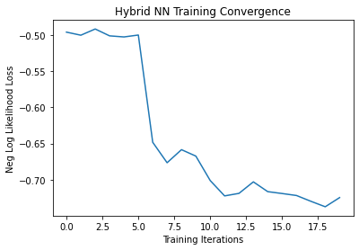
Somehow, the model’s loss converged a bit smoother than it did before, although a huge jump did occur in the first few iterations.
plt.plot(loss_list)
plt.title('Hybrid NN Training Convergence')
plt.xlabel('Training Iterations')
plt.ylabel('Neg Log Likelihood Loss')
Text(0, 0.5, 'Neg Log Likelihood Loss')
Testing Neural Network
Similarly, same process of testing the results as I did before, except having to decode 0 and 1 into 3s and 7s just for convenience.
model.eval()
with torch.no_grad():

    correct = 0
    for batch_idx, (data, target) in enumerate(test_loader):
        output = model(data)

        pred = output.argmax(dim=1, keepdim=True)
        correct += pred.eq(target.view_as(pred)).sum().item()

        loss = loss_func(output, target)
        total_loss.append(loss.item())

    print('Performance on test data:\n\tLoss: {:.4f}\n\tAccuracy: {:.1f}%'.format(
        sum(total_loss) / len(total_loss),
        correct / len(test_loader) * 100)
        )
Performance on test data:
	Loss: -0.7454
	Accuracy: 91.0%
n_samples_show = 8
count = 0
fig, axes = plt.subplots(nrows=1, ncols=n_samples_show, figsize=(10, 3))

model.eval()
with torch.no_grad():
    for batch_idx, (data, target) in enumerate(test_loader):
        if count == n_samples_show:
            break
        output = model(data)

        pred = output.argmax(dim=1, keepdim=True)

        axes[count].imshow(data[0].numpy().squeeze(), cmap='gray')

        axes[count].set_xticks([])
        axes[count].set_yticks([])
        axes[count].set_title('Predicted {}'.format(3 if pred.item() == 0 else 7))

        count += 1
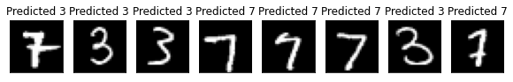
Notice that the model has achieved a lower testing accuracy due to numerous possible reasons, but details won’t matter.
Closing Remarks
Benefits of Hybrid Neural Networks
All the circuits we’ve used are classically simulatable, which means we’re not leveraging the potential of quantum computation, such as entanglement. The authors of the textbook also mentioned that the model would’ve trained equally, or even better without the quantum layer.
Without us utilizing quantum phenomenas/properties, the results will probably be similar to that of using a normal, classical neural network. However for now, we can always test out these kinds of networks to see if there are in fact possible benefits of using such kinds of network. It would require a more sophisticated quantum layer to possibly achieve greater “quantum advantage”.
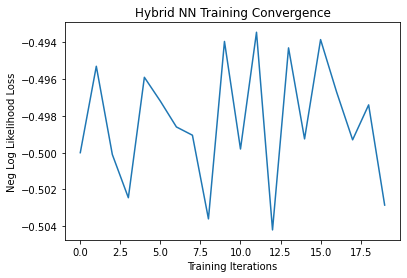
Experienced Issues
Although the results look reasonable here in this post, I did get questionable results in one of my earliest tries. Despite using a simulator, it seemed that the network at a certain trial didn’t learn, or the qubit’s results were just very unlucky after each measurement. The loss stayed at around $-0.5$ after 20 epochs, and achieved only 50% accuracy during testing - no better than a random guess. Here is the loss graph for the network I’ve just mentioned:
Overall Results
It’s very amusing to see how we can fuse quantum and classical layers together to create such neural networks, even if there’s no particular advantage of doing so. Regardless, we can always move up from here and apply the simpler concepts which the textbook has shown and see whether we can put hybrid NN to good use in the future!
Credits
Asfaw, A., Bello, L., Ben-Haim, Y., Bravyi, S., Capelluto, L., Vazquez, A. C., . . . Wootton, J. (2020). Learn Quantum Computation Using Qiskit. Retrieved from http://community.qiskit.org/textbook