Color Restoration with Generative Adversarial Network
Published:
Fast.ai has a two-part Deep Learning Course, the first being Practical Deep Learning for Coders, and the second being Deep Learning from the Foundations, both having different approaches and intended for different audiences. In the 7th lecture of Part 1, Jeremy Howard taught a lot about modern architectures such as Residual Network (ResNet) , U-Net, and Generative Adversarial Network (GAN).
Generative Adversarial Networks
GANs were first invented by Ian Goodfellow, one of the modern figures in the Deep Learning world. GANs could be used for various tasks such as Style Transfer, Pix2Pix, create CycleGAN, etc. Today what I’ll be experimenting with is Image Restoration.
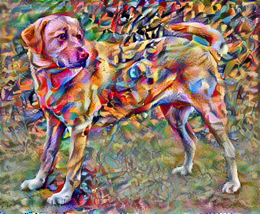
Image Restoration
There are different elements of an image which one can attempt to restore, and the example shown by Jeremy was restoring low resolution images into higher resolution images, which produces something like the following
Jeremy also mentioned that GANs would also be capable of not only restoring an image’s resolution, but other elements such as clearing JPEG-like artifacts, different kinds of noise, or even restoring colors. And with that, I immediately hooked to finish the lecture and try out what I’ve learned, and thus came this project.
Color Restoration
Instead of turning low resolution images to high resolution images, I instead wanted to build a network which will be able to recolor black and white images. The approach is to do so is still similar in terms of how a GAN works, except with a few tweaks which we’ll discuss further down.
Code Source
Since it is the first time I’ve worked with generative networks like GANs, I decided to base my code heavily on a fast.ai notebook, lesson7-superres-gan.ipynb.
The code provided below isn’t complete and only the important blocks of code were taken.
The GAN Approach
A GAN is sort of like a game between two entities, one being the artist (formally generator) and the other being the critic (formally discriminator). Both of them have their own respective roles: the artist has to produce an image, while the critic has to decide whether the image produced by the artist is a real image or a fake/generated image.
The two of them have to get better at what they do, the critic has to get better at differentiating real from fake images, while the artist has to improve the image produced to fool the critic. The implementation of this concept to a task like image restoration is pretty much like the aforementioned. That is, the artist has to produce a higher resolution image from the low resolution image, while the critic also learns to distinguish between the two possibilities.
Now, to apply that to color restoration, instead of differentiating low resolution from high resolution images, the critic has to classify artist-generated images from colored images, and while doing so the artist has to learn how to better recolor the images it produces to outsmart the critic.
Data Modification
In order to build a network that is able to both learn to recolor images and to classify real from fake images, we need to provide it two sets of data, namely a colored image and its corresponding black-and-white image. To do so, we used the Pets dataset from Oxford IIT which are colored, and created a function to grayscale the images. Jeremy called the function to do such task as a crappifier, which in our case only grayscales the images. Once we have our colored and grayscaled images, we can use it later to train the network.
from PIL import Image, ImageDraw, ImageFont

class crappifier(object):
    def __init__(self, path_lr, path_hr):
        self.path_lr = path_lr
        self.path_hr = path_hr

    def __call__(self, fn, i):
        dest = self.path_lr/fn.relative_to(self.path_hr)
        dest.parent.mkdir(parents=True, exist_ok=True)
        img = PIL.Image.open(fn)
        img = img.convert('L')
        img.save(dest, quality=100)
Pre-train Generator/Artist
Now, we will begin to train our generator first before using it in a GAN. The architecture we’ll use is a U-Net, with ResNet34 as its base model and all it’s trained to do is to recolor the images so it looks more like its colored-counterpart. Notice also that we’re using Mean Squared Error or MSELossFlat as our loss function.
arch = models.resnet34
loss_gen = MSELossFlat()

learn_gen = unet_learner(data_gen, arch, wd=wd, blur=True, norm_type=NormType.Weight,
                         self_attention=True, y_range=y_range, loss_func=loss_gen)
Once we have the generative model, we can train the model head for a few epochs, unfreeze, and train for several more epochs.
learn_gen.fit_one_cycle(2, pct_start=0.8)
| epoch | train_loss | valid_loss | time |
|---|---|---|---|
| 0 | 0.109306 | 0.111038 | 02:37 |
| 1 | 0.096312 | 0.102479 | 02:40 |
learn_gen.unfreeze()
learn_gen.fit_one_cycle(3, slice(1e-6,1e-3))
| epoch | train_loss | valid_loss | time |
|---|---|---|---|
| 0 | 0.089206 | 0.100583 | 02:41 |
| 1 | 0.087562 | 0.094716 | 02:44 |
| 2 | 0.086839 | 0.094106 | 02:45 |
The resulting generated images after a total of 5 epochs looks like the following
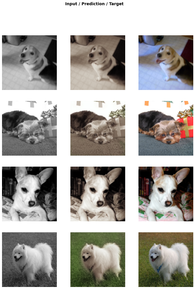
As you can see, the generator did poorly on some areas of the image, while it did great in others. Regardless, we’ll save those generated images to be used as the fake images dataset for the critic to learn from.
Train Discriminator/Critic
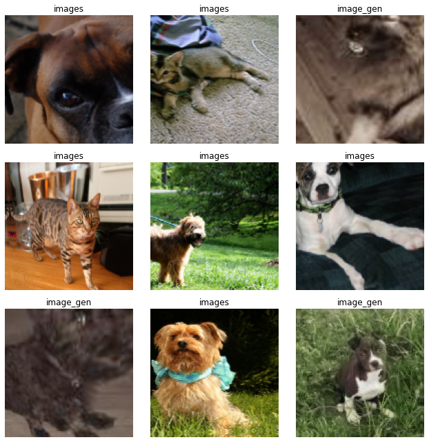
After generating two sets of images, we’ll feed the data to a critic and let it learn to distinguish between real images from the artist-generated images. Below is a sample batch of data, where the real images are labelled simply as images and the generated ones as image_gen
To create the critic, we’ll be using fast.ai’s built-in gan_critic, which is just a simple Convolutional Neural Network with residual blocks. Unlike the generator, the loss function we’ll use is Binary Cross Entropy, since we only have two possible predictions, and also wrap it with AdaptiveLoss.
loss_critic = AdaptiveLoss(nn.BCEWithLogitsLoss())

learn_critic = Learner(data_crit, gan_critic(), metrics=accuracy_thresh_expand, loss_func=loss_critic, wd=wd)
Once the Learner has been created, we can proceed with training the critic for several epochs.
learn_critic.fit_one_cycle(6, 1e-3)
| epoch | train_loss | valid_loss | accuracy_thresh_expand | time |
|---|---|---|---|---|
| 0 | 0.170356 | 0.105095 | 0.958804 | 03:34 |
| 1 | 0.041809 | 0.022646 | 0.992365 | 03:27 |
| 2 | 0.026520 | 0.013480 | 0.996638 | 03:26 |
| 3 | 0.011859 | 0.005585 | 0.999117 | 03:25 |
| 4 | 0.012674 | 0.005655 | 0.999288 | 03:25 |
| 5 | 0.013518 | 0.005413 | 0.999288 | 03:24 |
GAN
With both of the generator and the critic pretrained, we can finally use both of them together and commence the game of outsmarting each other found in GANs. We will be utilizing AdaptiveGANSwitcher, which basically goes switches between generator to critic or vice versa when the loss goes below a certain threshold.
switcher = partial(AdaptiveGANSwitcher, critic_thresh=0.65)
Wrapping both the generator and the critic inside a GAN learner:
learn = GANLearner.from_learners(learn_gen, learn_crit, weights_gen=(1.,50.), show_img=False, switcher=switcher,
                                 opt_func=partial(optim.Adam, betas=(0.,0.99)), wd=wd)
A particular callback we’ll use is called GANDiscriminativeLR, which handles multiplying the learning rate for the critic.
learn.callback_fns.append(partial(GANDiscriminativeLR, mult_lr=5.))
Finally, we can train the GAN for 40 rounds before we use a larger image size to train for another 10 rounds.
lr = 1e-4
learn.fit(40, lr)
| epoch | train_loss | valid_loss | gen_loss | disc_loss | time |
|---|---|---|---|---|---|
| 0 | 3.718557 | 3.852783 | 03:27 | ||
| 1 | 3.262025 | 3.452096 | 03:29 | ||
| 2 | 3.241105 | 3.499610 | 03:29 | ||
| 3 | 3.098072 | 3.511492 | 03:31 | ||
| 4 | 3.161309 | 3.211511 | 03:30 | ||
| 5 | 3.108723 | 2.590987 | 03:29 | ||
| 6 | 3.049329 | 3.215695 | 03:29 | ||
| 7 | 3.156122 | 3.255158 | 03:29 | ||
| 8 | 3.039921 | 3.255423 | 03:30 | ||
| 9 | 3.136142 | 3.109873 | 03:30 | ||
| 10 | 2.969435 | 3.096309 | 03:30 | ||
| 11 | 2.967517 | 3.532753 | 03:30 | ||
| 12 | 3.066835 | 3.302504 | 03:28 | ||
| 13 | 2.979472 | 3.147814 | 03:29 | ||
| 14 | 2.848181 | 3.229101 | 03:29 | ||
| 15 | 2.981036 | 3.370961 | 03:30 | ||
| 16 | 2.874022 | 3.646701 | 03:32 | ||
| 17 | 2.816335 | 3.517284 | 03:33 | ||
| 18 | 2.886316 | 3.336793 | 03:33 | ||
| 19 | 2.851927 | 3.596783 | 03:33 | ||
| 20 | 2.885449 | 3.560956 | 03:33 | ||
| 21 | 3.081255 | 3.357426 | 03:31 | ||
| 22 | 2.812135 | 3.340290 | 03:33 | ||
| 23 | 2.933871 | 3.475993 | 03:32 | ||
| 24 | 3.084240 | 3.034758 | 03:31 | ||
| 25 | 2.983608 | 3.113349 | 03:33 | ||
| 26 | 2.746827 | 2.865806 | 03:32 | ||
| 27 | 2.789029 | 3.173259 | 03:33 | ||
| 28 | 2.952777 | 3.227012 | 03:32 | ||
| 29 | 2.825185 | 3.053979 | 03:34 | ||
| 30 | 2.782907 | 3.444182 | 03:34 | ||
| 31 | 2.805190 | 3.343132 | 03:33 | ||
| 32 | 2.901620 | 3.299375 | 03:33 | ||
| 33 | 2.744463 | 3.279421 | 03:32 | ||
| 34 | 2.818238 | 3.048206 | 03:32 | ||
| 35 | 2.755671 | 2.975504 | 03:32 | ||
| 36 | 2.764382 | 3.075425 | 03:32 | ||
| 37 | 2.714343 | 3.076662 | 03:32 | ||
| 38 | 2.805259 | 3.291719 | 03:32 | ||
| 39 | 2.787018 | 3.172551 | 03:32 |
learn.data = get_data(16, 192)
learn.fit(10, lr/2)
| epoch | train_loss | valid_loss | gen_loss | disc_loss | time |
|---|---|---|---|---|---|
| 0 | 2.789968 | 3.127500 | 08:28 | ||
| 1 | 2.842687 | 3.226334 | 08:22 | ||
| 2 | 2.764777 | 3.127393 | 08:24 | ||
| 3 | 2.783910 | 3.183345 | 08:23 | ||
| 4 | 2.731649 | 3.279976 | 08:21 | ||
| 5 | 2.652934 | 3.143363 | 08:23 | ||
| 6 | 2.664248 | 2.998718 | 08:22 | ||
| 7 | 2.777635 | 3.185632 | 08:27 | ||
| 8 | 2.718668 | 3.357025 | 08:26 | ||
| 9 | 2.660009 | 2.887908 | 08:23 |
The resulting training images looks like the following
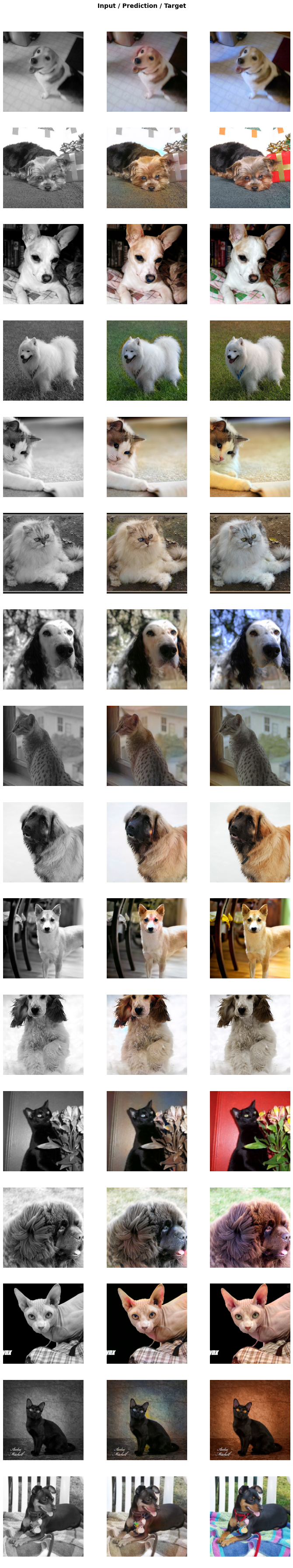
And as you can see, our model was able to recolor the images to a certain extent of accuracy. This is not bad, but GANs do have their weaknesses which we’ll discuss in the last section. Before we wrap up the GAN section, let’s try to feed the model external images, that is images that it hasn’t seen before.
Recoloring External Images
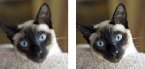
The following pet images were taken randomly from the internet. I’ve manually grayscaled the images and before letting the model predict its output.
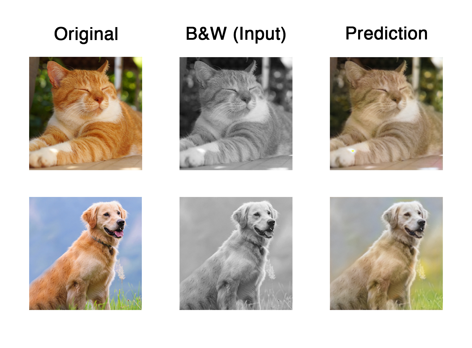
The colors produced, especially the animal’s fur is less saturated than it’s original image. However the natural background like grass and the sky is still acceptable, although different from the original.
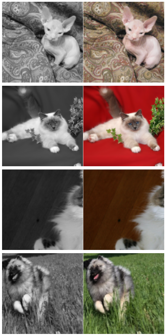
Lastly, I tried to feed an image which is not a cat nor a dog. I tried to feed it images of actual people. The top row is a black-and-white picture which is already grayscaled when I received it. Whereas the bottom row’s image went through the same process as the images right above.
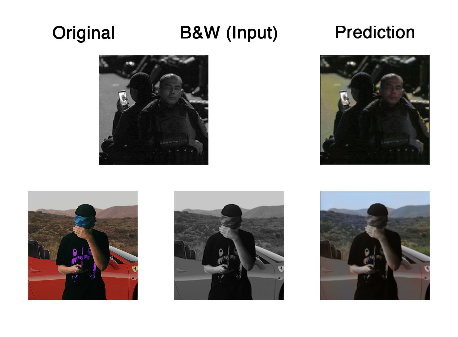
Few things to notice here for the first prediction, the model is biased towards green and yellow colors, hence the floor color of the first output. Secondly, aside from coloring the person in front, the model also colored the person on the phone’s screen.
On the other hand, the second prediction was great at coloring the backdrop of mountains and the sky, but is bad at coloring the supposedly bright-red car as well as coloring the person as it remained mostly grey.
The most likely reason behind the poor recoloring of a person is because of the dataset being used to train the GAN on, which are Pets in this case.
Closing Remarks
Weaknesses of GANs
GANs are well known for being troublesome to be handled, especially during training, hence the fancy configuration and knobs which we have to have in order for it to behave well. Moreover, they take quite long hours to train in comparison to other architectures.
Possible Replacement of GANs
Just like shown in the remaining of Lecture 7, there are other architectures which are as good or even better than GANs, one of which is to use Feature Loss coupled with U-Nets, with shorter training hours and better results in several cases. I have tried doing that approach, but will not be discussing that here.
Conclusion
GANs are great, the tasks they can do vary from one architecture to another, and is one of the methods to let a model “dream” and have their own forms of creativity. However, they have certain weaknesses which includes long training time and careful tweaking requirements. They are definitely modern, and doing reasearch in the domain is still very much open and fun to do if you’re into this particular field.
That’s it! Thanks for your time and I hope you’ve learned something!